Efficiency
- Time Efficiency (Computational/Temporal Complexity)
- Space Efficiency (Spatial Complexity)
We use a function ( τ ) for the actual execution time:
The execution time ( τ ) of an algorithm depends on its structure, the operations of the machine, and the data structures used. To compare two algorithms ( A ) and ( B ), we compare ( τA ) and ( τB ).
What could ( τ(n) ) depend on?
- The size ( n ) of the input
- Specific instances of the input
- The executor of the algorithm; computers that are more or less performant
Recap of Some Basic Math Concepts:
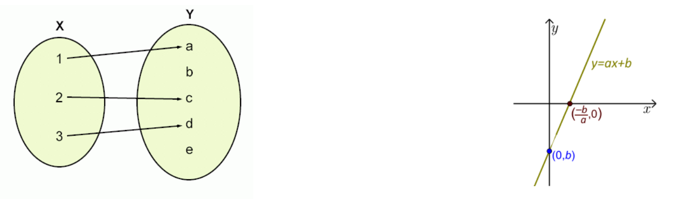
A function is a relationship that associates each element of a starting set (domain (X)) with an element of an arrival set (codomain (Y)).
The function is written as (f: X -> Y), where (y = f(x)) denotes the element (y ∈ Y) associated with (x ∈ X).
Functions represent the functional dependency between different quantities.
Functions can be visualized with a graph, showing pairs ((x, y)) on the Cartesian plane, where (y = f(x)).
Execution Times
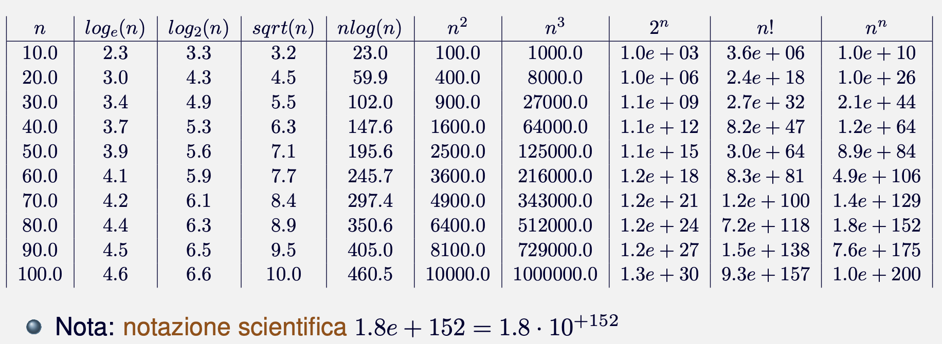
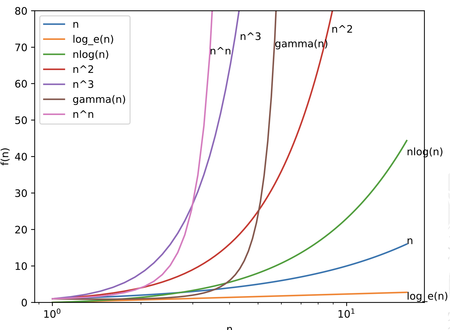
The execution times of algorithms can be expressed as univariate functions in relation to the size ( n ) of the input, denoted by (τ(n)). The functions are grouped into different categories based on their growth as ( n ) varies:
-
Less than linear
These execution times grow more slowly than a linear function:- Constant ( k ): the time does not vary with ( n ); the algorithm always takes the same time regardless of the size of the input.
- Logarithmic ( log_e(n) ) or $ \log_2(n) $: the execution time increases slowly with ( n ); typical of algorithms that reduce the input at each step, such as binary search.
-
Linear
- ( k * n ): the execution time grows proportionally to the size of the input. If ( n ) doubles, the time also doubles. This is typical of algorithms that need to visit every element once, like traversing a list.
-
More than linear
These execution times grow more rapidly than a linear function:- Linear-logarithmic ( n * log(n) ): common in efficient sorting algorithms like Merge Sort and Heap Sort.
- Polynomial ( n^k ): the time grows rapidly with ( n ) as ( k ) increases; typical of algorithms like Bubble Sort (( n^2 )).
- Exponential ( k^n ): the growth is extremely rapid; typical of algorithms that explore all possible combinations, such as some optimization problems.
- Factorial ( n! ) and super-exponential ( n^n ): grow much more quickly and are generally impractical for large values of ( n ).
These categories help to understand how scalable and efficient an algorithm is concerning the size of the input.
Execution Cases for a Fixed Size
For a fixed size ( n ), three possible cases are distinguished:
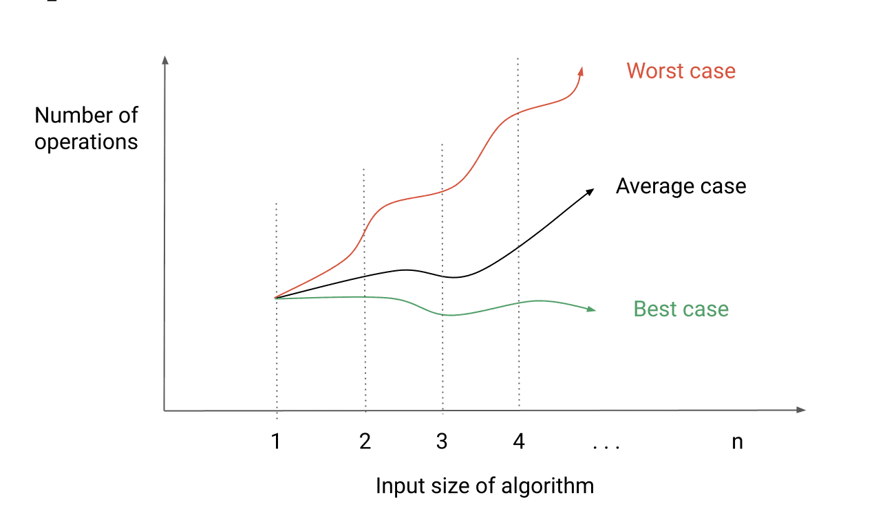
Algorithm Complexity Cases
-
Best Case: The input configurations that lead to the minimum execution time for an algorithm. For example, in a linear search algorithm, the best case occurs when the target element is the first item in the list. This case represents the fastest possible execution time for the algorithm.
-
Average Case: The input configurations considered "normal" or most commonly encountered in practice. This case represents the expected time complexity for typical inputs rather than extreme ones. The average case provides a realistic measure of an algorithm's efficiency under standard conditions.
-
Worst Case: The input configurations that lead to the maximum execution time. This scenario represents the upper bound on the time complexity, showing how the algorithm performs under the most demanding conditions. For instance, in sorting algorithms, the worst case might involve a completely reversed list.
Note on
These cases can vary significantly based on specific instances and on hardware and software factors, as different input configurations and system characteristics can heavily influence execution times.
However, algorithm analysts are generally more interested in how the execution time behaves as the input size ( n ) grows, rather than in the absolute times. The three different execution times, denoted as τ1(n) for the best case, τ2(n) for the average case, and τ3(n) for the worst case, may follow the same growth pattern (e.g., linear):
τ(n) = c_1n + c_2
An algorithm ( A ) might have lower absolute times than another algorithm ( B ) for small input sizes, or for specific cases, but it could have a worse growth rate as ( n ) increases, especially in the average case.
Computational Complexity and Efficient Algorithms
Computational complexity is defined as the order of magnitude of the function T(n).
Definition: Efficient/Inefficient Algorithms
An algorithm is defined as efficient if it has polynomial or sub-polynomial complexity.
In contrast, an algorithm is inefficient if it has super-polynomial complexity, such as exponential complexity. These algorithms tend to have execution times that grow rapidly with n , making them impractical for large inputs.
Asymptotic analysis
Asymptotic Efficiency
Asymptotic efficiency: is studied as the input size ( n ) tends to infinity (i.e., for values where only the order of growth is relevant). This approach allows us to focus on how the algorithm's time complexity grows with increasingly large inputs, ignoring minor constants and lower-order terms.
Asymptotic Execution Time: This is an approximation of an algorithm's execution time using a "simpler" function of the same order of growth, which provides a clearer view of the dominant trend without unnecessary detail.
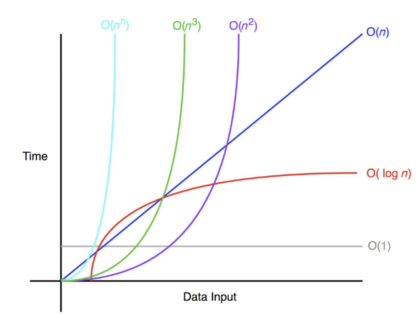
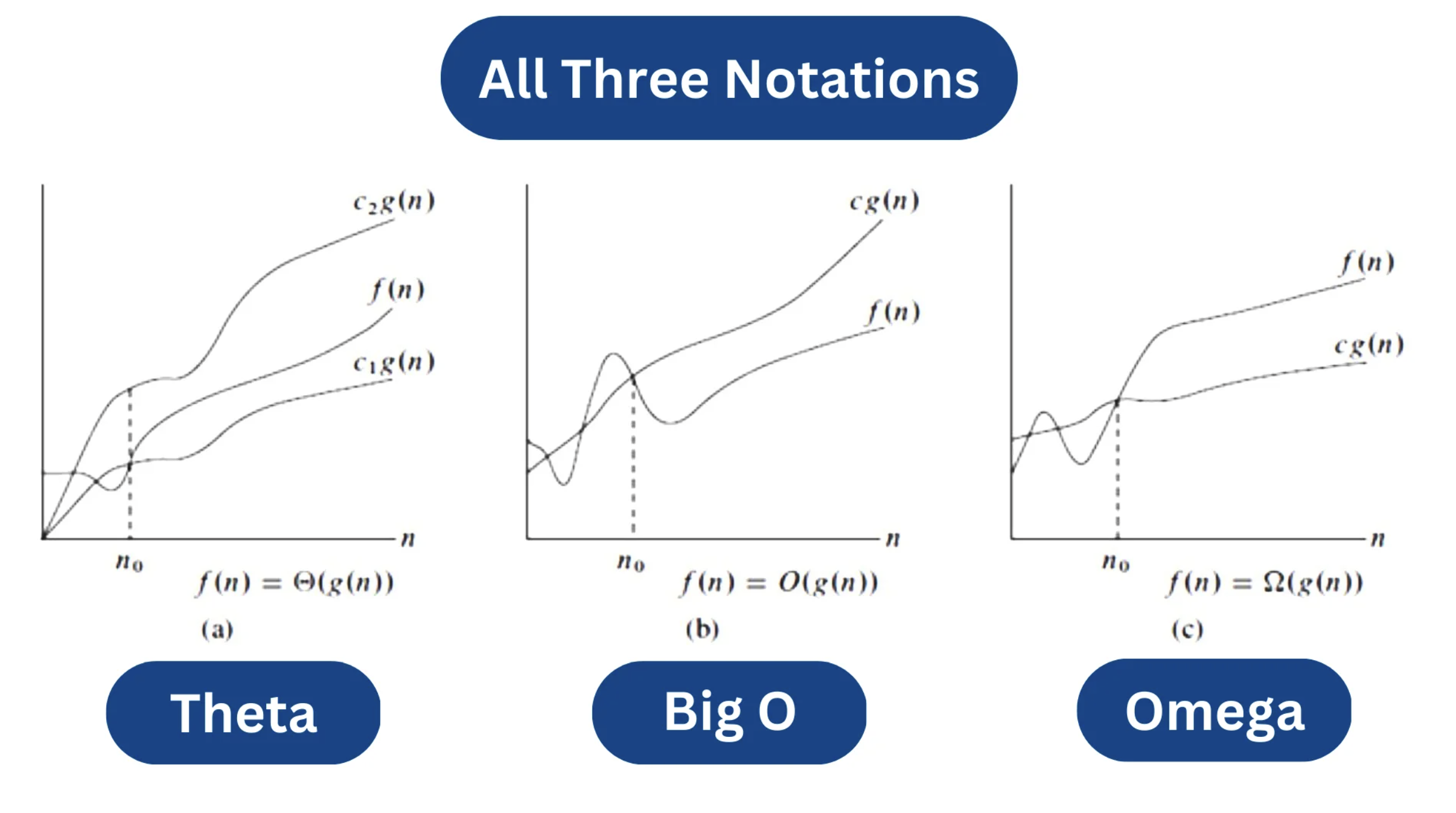
Big O, Big Omega, and Big Theta Notation
In algorithm analysis, we use Big O (O), Big Omega (Ω), and Big Theta (Θ) notation to describe the growth rate of functions. Each notation helps us understand how a function behaves as the input size increases.
Big O: This represents the worst-case performance for an algorithm, setting an upper bound on how slow your code can be. It’s noted as O(n²).
This upper bound indicates that, no matter the input, the algorithm’s runtime will not grow faster than n² as the input size increases.
Big Theta (Θ): This represents the average, typical case performance for an algorithm. It’s noted as Θ(n×p).
and provides a tight bound, meaning it defines both an upper and lower bound for the algorithm’s runtime, showing that the runtime grows asymptotically at the same rate as n×p as the input size increases.
Big Omega (Ω): This represents the best case performance for an algorithm, setting a lower bound on how fast the code can perform. It’s noted as Ω(n).
This lower bound indicates that, even in the best-case scenario, the algorithm’s runtime won’t be faster than n as the input size grows.